Math Linear Systems
A complete 24-session SAT® Algebra course for mastering linear systems: intersections, substitution, elimination, one/no/infinite solution cases, parameter problems, fractions and decimals, mixture, rate, cost, ticket, age, and multi-step word-problem modeling, three-variable systems, inequalities, function notation, data and graph interpretation, common-error correction, and digital SAT® strategy. Every session includes an explanatory diagram, six fully worked step-by-step examples, and 15 original SAT®-style multiple-choice practice questions, plus a cumulative 46-question final exam covering the whole course.
📚 Course Curriculum
Introduction. Welcome to Math Linear Systems. This first session sets the foundation for every session that. follows: what a system of linear equations actually is, …
🔒 Enroll to unlock this session.
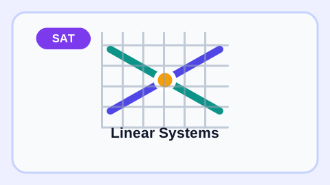
Introduction. Before you solve a system with algebra, it helps to recognize what a solution looks like when. it is shown to you directly — …
Open trial session →Introduction. Substitution is often the fastest way to solve a system when one equation is already solved for. a variable, or can be rearranged into …
🔒 Enroll to unlock this session.
Introduction. Elimination is often faster than substitution when neither equation is already solved for a. variable, but the coefficients line up (or can be scaled …
🔒 Enroll to unlock this session.
Introduction. So far every system in this course has had exactly one solution. But the SAT® frequently tests. whether you can tell, often without fully …
🔒 Enroll to unlock this session.
Introduction. Building on solution counts, this session focuses on problems where a coefficient is an unknown. letter (commonly \(k\), \(p\), or \(m\)) and you must …
🔒 Enroll to unlock this session.
Introduction. Systems do not always arrive with whole-number coefficients. This session shows how to turn a. system with fractions or decimals into an equivalent whole-number …
🔒 Enroll to unlock this session.
Introduction. Some systems don't have matching or opposite coefficients right away. This session covers how. to choose a scaling factor — often the least common …
🔒 Enroll to unlock this session.
Introduction. This session begins the modeling stage of the course: turning a word problem into a system. Mixture and investment problems share one repeatable structure …
🔒 Enroll to unlock this session.
Introduction. This session models situations with two moving objects — such as two vehicles, or one person. walking toward another — as a linear system …
Open trial session →Introduction. This session applies linear systems to business-style models: a cost function, a revenue. function, and the "break-even point" where a company's revenue exactly covers …
🔒 Enroll to unlock this session.
Introduction. This session extends cost-comparison modeling to ticketing and multi-tier fee situations, where. two categories of items (such as adult and student tickets) combine into …
🔒 Enroll to unlock this session.
Introduction. Age and number problems describe two related quantities at different points in time, or under. different conditions, and ask you to find their current …
🔒 Enroll to unlock this session.
Introduction. This session generalizes every modeling skill so far into one repeatable four-step process for. any multi-sentence word problem: read for two unknowns, define variables, …
🔒 Enroll to unlock this session.
Introduction. This session extends everything you have learned to a third equation and a third unknown. The. core idea does not change: you are still …
🔒 Enroll to unlock this session.
Introduction. Replacing the equals sign with an inequality changes a single-point solution into a whole. region of solutions. This session shows how to graph two …
🔒 Enroll to unlock this session.
Introduction. This session reframes everything you already know about systems using function notation. If. \(f(x)\) and \(g(x)\) are both linear, then solving \(f(x)=g(x)\) is exactly …
🔒 Enroll to unlock this session.
Introduction. This session trains you to notice shortcuts: systems where one equation is a clear multiple of. another, or where symmetric structure lets you skip …
Open trial session →Introduction. Solving a system correctly is only half the job on a word-problem question — you must also. state what the resulting coordinates mean in …
🔒 Enroll to unlock this session.
Introduction. Real data rarely arrives as a clean equation. This session shows how to build a linear model. from a data table or scatterplot and …
🔒 Enroll to unlock this session.
Introduction. This session ties together every representation you have used throughout the course — equation,. table, graph, and words — by practicing translation among all …
🔒 Enroll to unlock this session.
Introduction. This session catalogs the specific mistakes that cost the most points on linear-systems. questions, based on the setup, algebra, solution-count, and context slips seen …
🔒 Enroll to unlock this session.
Introduction. This session pulls together every method from the course — substitution, elimination, graphing,. tables, and backsolving — into one decision process for choosing the …
🔒 Enroll to unlock this session.
Introduction. This final session brings together every skill from the course in mixed, cumulative practice,. using a five-step mastery protocol to approach any linear-systems question …
🔒 Enroll to unlock this session.
Course Syllabus
Course Structure
This complete SAT® Math course contains 24 sessions organized into six stages, taking
linear systems from a first definition through real-world modeling, extended structures, and
full test-day strategy.
Stage 1: Foundations of Linear Systems
- What a Linear System Means — Identify a system, interpret the solution as an
intersection point, and check candidate solutions in both equations. - Reading Systems from Graphs and Tables — Locate a system's solution from a graph or a
table of values without solving algebraically first. - Substitution Method Mastery — Solve systems efficiently by replacing one variable with
an equivalent expression. - Elimination Method Mastery — Add, subtract, or scale equations to cancel a variable.
Stage 2: Solution Structure and Special Cases
- One, No, or Infinitely Many Solutions — Compare slopes and intercepts to classify a
system without fully solving it. - Parameter Problems — Find the unknown coefficient that forces a specific solution count.
- Systems with Fractions and Decimals — Clear denominators and decimals before solving.
- Strategic Scaling and Multi-Step Elimination — Choose the least common multiple of two
coefficients to eliminate a variable in one clean step.
Stage 3: Real-World Modeling
- Mixture and Investment Problems — Build a count equation and a value equation from a
blended quantity. - Rate, Distance, and Time Problems — Model two travelers with linear distance functions.
- Cost, Revenue, and Break-Even Models — Compare fixed and variable costs to find a
break-even point. - Ticket, Fee, and Plan-Comparison Problems — Translate two pricing plans into a system.
- Age and Number Relationship Problems — Track two related quantities across time or
conditions. - Translating Word Problems into Systems — Convert a multi-sentence scenario into two
linear equations and interpret the answer in context.
Stage 4: Extended Structures
- Three-Variable Linear Systems — Extend elimination to a third equation and unknown.
- Systems of Linear Inequalities — Find the region satisfying two linear inequalities.
- Function Notation and Linear Systems — Interpret f(x) = g(x) as a system.
- Systems with Special or Repeated Structure — Recognize multiples, symmetry, and
shortcuts that avoid unnecessary computation.
Stage 5: Graphs, Data, and Representation
- Interpreting Intersection Points in Context — Translate a coordinate pair into a
real-world statement with correct units. - Systems from Data Tables and Scatterplots — Build linear models from recorded data and
find where two trends meet. - Multiple Representations — Move fluently between equation, table, graph, and words.
Stage 6: Test-Day Mastery
- Common Errors and Misconceptions — Diagnose and correct the mistakes that cost the
most easy points. - Digital SAT® Strategy — Choose efficiently among algebra, graphing, tables, and
backsolving. - Mixed Mastery Review and Final Exam Preparation — Apply a repeatable decision process
to cumulative, mixed practice.
Recommended Study Routine
Complete the sessions in order. For each session, read the Introduction, Definition,
Real-Life Uses, and Why You Should Know This sections, study all six worked examples, then
complete that session's 15 multiple-choice questions without notes. Review every explanation
before moving on, and keep a running error log grouped by setup errors, algebra errors,
solution-count errors, and context errors.
Session Assessment
Every session includes 15 SAT®-style multiple-choice questions linked directly to that
lesson, moving from direct computation to multi-step reasoning and context interpretation. A
cumulative 46-question final exam draws on every session to check whole-course mastery
before test day.
Course Outcomes
By the End of This Course, You Will Be Able To
- Explain what a linear system's solution represents and verify a candidate solution in both
original equations. - Read a system's solution directly from a graph or a table of values.
- Solve two-variable linear systems by substitution and by elimination, choosing the faster
method for a given setup. - Classify a system as having one, no, or infinitely many solutions by comparing slopes and
intercepts. - Find parameter values that force a specific number of solutions.
- Clear fractions and decimals from a system before solving it.
- Scale equations strategically to eliminate a variable in the fewest possible steps.
- Model mixture, investment, rate-distance-time, cost-revenue, plan-comparison, and age
problems as linear systems. - Translate a multi-sentence word problem into two linear equations and answer the exact
quantity requested. - Extend elimination to three-variable systems.
- Find the solution region of a system of linear inequalities.
- Interpret f(x) = g(x) as a system and locate the crossing point of two functions.
- Recognize special structure, such as one equation being a multiple of another, to shortcut
unnecessary algebra. - Interpret an intersection point's coordinates as a real-world statement with correct units.
- Build linear models from data tables and scatterplots and find where two trends meet.
- Move fluently between equation, table, graph, and verbal representations of the same system.
- Diagnose and correct common errors, including sign slips, partial scaling, and reporting the
wrong variable. - Choose confidently among algebra, graphing, tables, and backsolving on the digital SAT®.
- Complete a cumulative, mixed 46-question exam covering every session with improved accuracy
and time management.
📝 Practice Questions
406 interactive questions with instant feedback and explanations.
Enroll for free to unlock the full practice bank after the trial sessions.